Phase Field Modelling
Abstract
Abstract
1. INTRODUCTION
Material properties and its behaviour are fundamentally governed by the laws of physics. Given the accuracy-cost trade off, the most reliable method for modeling the evolution of a material state in mesoscale is by finding the numerical solution for Phase Field equations. In recent years, phase field models are extensively employed to model microstructural evolution in a wide variety of systems which include study of microstructural evolution during solidification, solid-solid phase transformations and plastic deformation. In this project, we primarily focussed on modelling solid-solid transformations. All the computations were carried out using python and in the due process we realised the usage of computational tools for solving mathematical models which govern the kinetics of a materials system.
2. METHODOLOGY
A. Materials Science Aspect
Phase is a physically, distinct, chemically homogeneous, mechanically separable part of a system. In a rudimentary level it can be classified as solid, liquid and gas. When pure systems are mixed together, they can exhibhit different phases depending on the composition and temperature. A mapping between the stability of a given phase with the corresponding composition and temperature can be studied using a phase diagram, which in turn could be obtained using various methods such as Cooling Curves, Thermodynamics, X-ray diffraction etc. In this project, Thermodynamical approach was used. Miscibility gap and order disorder transformations appearing in a phase diagram are simulated with the aid of computer program. Further we discuss about Fick’s law of diffusion and limitations of classical diffusion. We go through the solution of classical diffusion equations using analytical and numerical methods. It turns out that, considering Free energy as a "functional” resolves the limitation. Mathematical models namely Cahn-Hilliard and Allen-Kahn equations are derived and solved using numerical methods, and Gibbs thompson effect is also incorporated into the models. Using these models we simulated the spinodal decomposition, grain growth and precipitate growth.
B. Mathematical model
Governing equations for the given problem are Cahn-Hilliard equation, Allen-Kahn equation and Euler-Lagrange equation.
Cahn-Hilliard Equation:

Where;
C is concentration
t is time
M is mobility constant
κ is a constant
Allen-Kahn equation:

Where;
Φ is the ordering parameter
Euler-Lagrange Equation:

C. Computational aspect:
The above mentioned models were solved using analytical and numerical methods. In numerical methods we used implicit and explicit spectral techniques and by comparison we get better result with semi-implicit model which allows larger time steps. These are solved using python by exploiting libraries such as numpy, and SciPy. Computations were done using above models in representative area elements by putting appropriate boundary conditions. Matplotlib was used for plotting all the curves and simulations.
3. RESULTS

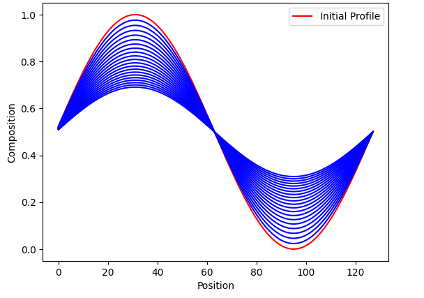
Explicit periodic boundary condition 1D solution of the diffusion equation

Solution of classical diffusion equation

Solution of Cahn-Hilliard diffusion equation

3D implementation of Cahn-Hilliard equation

2D implementation of Alen-Cahn equation

Gibbs Thomson effect
4. CONCLUSION
In this project, we first explored concepts of introductory metallurgical thermodynamics and Fick’s laws of diffusion and then extended those concepts to understand spinodal decomposition and its dependency on composition. We then looked at the solution for the classical diffusion equation using analytical and numerical methods by considering different boundary conditions and realised the reason for its failure. The spinodal region was plotted in Python using the classical diffusion equation, and we could see its inability to explain the phase separation. We then looked at the free energy functional and how it can be used to derive the Cahn-Hilliard (CH) equation. Solutions to the CH equation were obtained using numerical methods,
such as the finite difference method and the spectral method. We also looked at the derivation of the Allen-Cahn (AC)
equation. The solutions of the CH and AC equations were then implemented with different boundary conditions to obtain the simulations of 2D spinodal decomposition, Grain growth, and Precipitate growth, and we could observe that the CH and AC successfully model these situations and overcome the failure of the classical diffusion equation.
5. REFERENCES
[1] Phase Transformations in Metals and Alloys ByDavid A. Porter, Kenneth E. Easterling, Mohamed Y. Sherif
[2] Advanced Engineering Mathematics By Erwin Kreyszig.
[3] Python Crash Course, 2nd Edition: A Hands On, Project Based Introduction to Programming by Eric Matthes
Report Information
Team Members
Team Members
Report Details
Created: March 21, 2024, 6:53 p.m.
Approved by: Sukrit Dass T M [Piston]
Approval date: March 22, 2024, 2:15 p.m.
Report Details
Created: March 21, 2024, 6:53 p.m.
Approved by: Sukrit Dass T M [Piston]
Approval date: March 22, 2024, 2:15 p.m.

