Aim : 

The primary aim of this project is:

To develop a physically accurate, closed-loop dynamic simulation model of an 81-rack multi-zone building HVAC system in MATLAB/Simulink and to analyze its thermal performance and control behavior under the given ambient and architectural conditions.

The specific objectives are:

•  To model exponential airflow velocity decay with distance from the fan unit using the decay equation V = V₀ × e^(−0.05x).
•  To compute the convective heat transfer coefficient h for each rack using the Reynolds number, Nusselt number correlation, and air thermophysical properties.
•  To implement an energy balance integrator for each rack with a physically meaningful initial condition (T₀ = 25°C) and thermal gain.
•  To aggregate temperatures from 81 racks using a two-stage MinMax tree to identify the worst-case (hottest) rack driving the control loop.
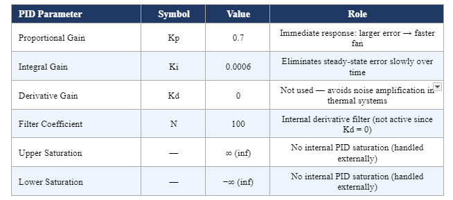
•  To design and implement a PID controller (Kp = 0.7, Ki = 0.0006, Kd = 0) for fan speed regulation with a 27°C setpoint.
•  To incorporate a Hysteresis block preventing chattering and a Saturation block enforcing the physical fan speed limit of 0–13 m/s.
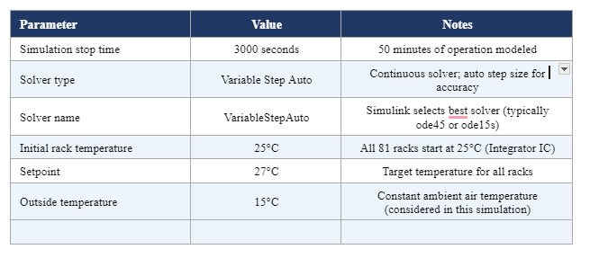
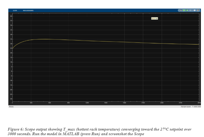
•  To simulate the complete closed-loop system for 3000 seconds using a variable-step continuous solver and observe temperature convergence.

Introduction : 

Modern buildings represent one of the largest sectors of global energy consumption, accounting for approximately 40% of total primary energy use worldwide. Within this, Heating, Ventilation, and Air Conditioning (HVAC) systems are typically responsible for 50–60% of a building’s energy consumption, making their efficient design and control one of the highest-impact areas in building energy management. As buildings grow in scale and complexity — incorporating server racks, open-plan offices, and large commercial spaces — the challenge of maintaining thermal comfort across multiple zones while minimizing energy use becomes increasingly significant.

A multi-zone HVAC system distributes conditioned air from a central unit through a duct network to multiple racks or zones. Unlike single-zone systems, multi-zone architectures must contend with spatial variation in airflow, distance-dependent losses in air velocity, and differential heat loads across zones. The rack farthest from the fan receives the weakest airflow and thus the least cooling — a physical reality captured in this model through the exponential decay law V = V₀ × e^(−0.05x), where x is the distance from the fan. This distance-dependent airflow is then translated into a convective heat transfer coefficient using established flat-plate boundary layer theory, grounding the simulation in fundamental fluid mechanics.

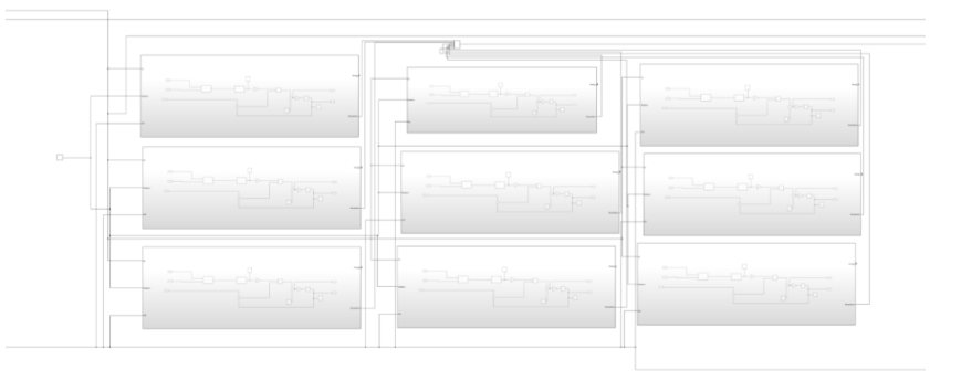
MATLAB/Simulink provides an ideal platform for developing such models. Its block-diagram paradigm naturally maps onto the modular structure of a building’s thermal zones, and its rich library of blocks — integrators, MATLAB Function blocks, PID controllers, Scope monitors, and Stateflow charts — allows both continuous-time physics and discrete control logic to coexist within a single model. This project leverages these capabilities to build an 81-rack model (Subsystems 74–161) organized as 9 clusters of 9 racks, connected to a central PID-controlled fan.

The control problem is as follows: given that outside air temperature is varying and the target rack temperature is 27°C, determine the fan speed V₀ (m/s) that maintains all racks at or near setpoint. Because not all racks receive the same airflow, the controller uses the maximum temperature across all 81 racks as its feedback signal — ensuring that even the worst-served rack remains within acceptable bounds. A PID controller continuously adjusts fan speed based on the error between setpoint and this maximum temperature, while a Hysteresis block prevents rapid oscillation and a Saturation block enforces the physical limit of 13 m/s.

Literature Survey : 

D.1 Overview of Building HVAC Modeling and Control

The literature on HVAC system modeling and control spans several decades and covers both theoretical foundations and practical implementations. Seminal works in building thermal modeling use lumped-parameter approaches — also called RC thermal networks — where each rack is represented as a thermal capacitance exchanging heat with adjacent zones and the outdoor environment through resistances. This approach underlies the integrator-based rack model used in this project, where the thermal mass (capacitance) is set to 500 J/K and the heat input is the convective energy from the fan-driven airflow.

PID control remains the industry standard for HVAC temperature regulation due to its simplicity, robustness, and well-understood tuning procedures. Studies have consistently demonstrated that well-tuned PID controllers can maintain rack temperatures within ±0.5°C of setpoint under typical disturbances. The proportional gain determines the immediate response to temperature error, the integral gain eliminates steady-state offset, and the derivative gain (often set to zero in HVAC applications to avoid noise amplification) dampens oscillations. This project uses Kp = 0.7 and Ki = 0.0006, with Kd = 0, consistent with the slow thermal dynamics of building zones.

D.2 Forced Convective Heat Transfer in Duct and Rack Airflow

The heat transfer between fan-driven air and rack surfaces is governed by forced convection. For external flow over flat surfaces — a reasonable approximation for airflow across server racks, walls, or ceiling panels — the local and average Nusselt number depends on the flow regime (laminar or turbulent) as characterized by the Reynolds number.

For laminar flow (Re < 5 × 10⁵) over a flat plate, the correlation is:

Nu = 0.664 × Re^0.5 × Pr^ (1/3) [Laminar, Re < 5×10⁵]

For turbulent or mixed boundary layer conditions (Re ≥ 5 × 10⁵):

Nu = (0.037 × Re^0.8 − 871) × Pr^ (1/3) [Turbulent/Mixed, Re ≥ 5×10⁵]

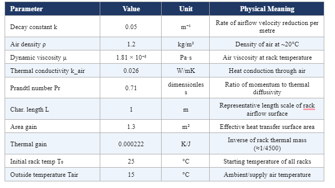
These correlations (from Incropera et al., Fundamentals of Heat and Mass Transfer) are directly implemented in the MATLAB Function block labeled ‘h’ inside each rack subsystem, using air properties ρ = 1.2 kg/m³, μ = 1.81 × 10⁻⁵ Pa·s, k_air = 0.026 W/mK, and Pr = 0.71 — all at standard rack temperature. The resulting h value (W/m²K) characterizes how effectively the airflow transfers heat to or from the rack.

D.3 Exponential Airflow Decay in Duct Networks

In real HVAC duct networks, air velocity decreases with distance from the fan due to frictional losses, turbulent mixing, and leakage. For simplified models, this decay is often approximated as exponential: V(x) = V₀ × e^(−kx), where k is a decay constant depending on duct geometry and roughness. This model is used extensively in building simulation tools including EnergyPlus and TRNSYS for variable-air-volume (VAV) systems.

In this project, k = 0.05 m⁻¹ is used, meaning airflow decays to approximately 60% of its source value at 10 m distance and to 37% at 20 m. This is a physically reasonable approximation for smooth ductwork at moderate velocities. The three rack distances in each cluster (2 m, 4 m, 6 m) correspond to velocity retentions of approximately 90%, 82%, and 74% of V₀ respectively.

D.4 Hysteresis Control in HVAC Systems

Hysteresis (or bang-bang with dead band) control is a fundamental technique in HVAC systems to prevent ‘chattering’ — the rapid on-off cycling of actuators (fans, valves, compressors) that would otherwise occur when the controlled variable hovers near the setpoint. By introducing upper and lower switching thresholds (the hysteresis band), the controller avoids unnecessary switching and extends equipment life.

In this model, the Hysteresis block is implemented as a MATLAB Function using a persistent state variable. The cooling system operates in free-cooling mode while the outside air temperature remains below 8 °C, using ambient air directly for cooling. Once the outside temperature rises above 10 °C, the system switches to compressor mode, maintaining the supply air at 10 °C. The 8–10 °C hysteresis band prevents rapid switching between operating modes due to small temperature fluctuations.

D.5 Multi-Zone Control and Worst-Case Temperature Feedback

A key design choice in multi-zone HVAC control is determining which zone’s temperature to use as the feedback signal. Using the average temperature can leave the hottest zone underserved; using individual zone controllers requires multiple actuators. A practical compromise — used in this project — is to feed back the maximum (worst-case) temperature across all zones to a single central controller. This ensures that even the most thermally stressed rack remains within acceptable bounds, at the cost of potentially overcooling some other racks.

The two-stage MaxTree implementation (nine intermediate Max10–Max18 blocks each aggregating 9 racks, followed by a final Max19 block aggregating the nine intermediate maxima) is an efficient.

E.1 System Architecture Overview

The Simulink model implements a complete closed-loop HVAC control system for an 81-rack building. The architecture consists of five layers: (1) Input signals, (2) Rack thermal subsystems, (3) Temperature aggregation, (4) PID control loop, and (5) Feedback to racks. Each layer is described in detail below, with all parameter values extracted directly from the model.

E.2 Input Signals

The model has three primary input signals that feed into the rack subsystems and control loop:

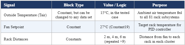
The three distance values (Constants 10, 11, 12 — and repeated for each subsequent group) directly feed the airflow decay MATLAB Function block inside each rack subsystem. Racks at 2 m receive the strongest airflow; racks at 6 m receive the weakest.

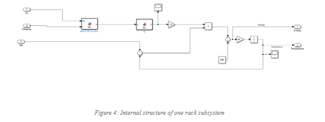
E.3 Rack Thermal Subsystem

Each of the 81 racks is modeled as an identical Simulink subsystem (Subsystems 74–161) with three inputs and two outputs:

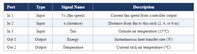
Inside each rack subsystem, four computational blocks operate in sequence:

E.3.1 Step 1 — Airflow Velocity Decay

The first MATLAB Function block computes the actual air velocity reaching the rack from the fan speed and the rack’s distance:

The complete MATLAB function as implemented in the model:

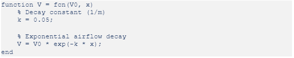
At Kp = 0.05 m⁻¹, a rack at x = 2 m receives V = V₀ × e^(−0.1) ≈ 0.905 V₀ (90.5%), at 4 m receives 0.819 V₀ (81.9%), and at 6 m receives 0.741 V₀ (74.1%). This ensures racks farther from the fan receive realistically weaker airflow.

E.3.2 Step 2 — Convective Heat Transfer Coefficient h(V) :

The second MATLAB Function block converts the local air velocity V into a convective heat transfer coefficient h using flat-plate boundary layer theory. The implementation:

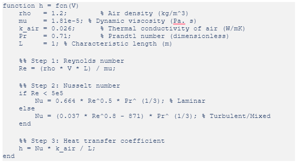
The physical reasoning behind each step:

• Reynolds number Re = ρVL/μ characterizes the flow regime. For typical fan speeds of 5–13 m/s with L = 1 m, re ≈ 3.3×10⁵ to 8.6×10⁵, placing flow in the mixed regime.
• Nusselt number Nu represents the ratio of convective to conductive heat transfer. The two-branch correlation (0.664 × Re^0.5 for laminar, 0.037 × Re^0.8 − 871 for turbulent) is the standard flat-plate formula from Incropera et al.

Heat transfer coefficient h = Nu × k_air / L, in W/m²K, gives the rate of heat exchange per unit area per degree of temperature difference

E.3.3 Step 3 — Rack Energy Balance

The heat energy transferred to the rack per unit time (power, in Watts) is:

Where:

• Gain_area = 1.3 (the Gain block in the subsystem, representing effective heat transfer area in m²)
• T_air = 15°C (outside temperature, can be changed to varying)
• T_rack = current rack temperature (fed back from the integrator output)

The temperature difference (Tair − Track) is computed by the Sum2 block (configured as −+). When the rack is warmer than outside air, this drives heat removal from the rack (cooling effect).

E.3.4 Step 4 — Temperature Integrator

The energy Q is integrated over time to compute rack temperature. A Gain block (Gain1 = 0.000222) scales the energy signal to represent the inverse of thermal mass:

The Integrator block has an initial condition of T₀ = 25°C, representing racks that start at 25°C before the system is switched on. The factor 0.000222 corresponds to 1/Thermal_mass ≈ 1/4500 J/K, the effective thermal capacitance of the rack air and contents.

E.4 Temperature Aggregation — Two-Stage Max Tree

With 81 rack subsystems each outputting a Temperature signal, the system needs to identify the single hottest rack to feed back to the PID controller. Since Simulink’s MinMax block accepts a maximum of 9 inputs, the aggregation is implemented as a two-stage tree:

• Stage 1: Nine intermediate Max blocks (Max10 through Max18), each receiving 9 rack temperatures and outputting a single maximum value. This produces 9 intermediate maxima.
• Stage 2: One final Max block (Max19) receives the 9 intermediate maxima and outputs T_max — the temperature of the single hottest rack across the entire building.

This T_max value is the feedback signal for the PID controller. By controlling for the worst-case rack, the system guarantees that no rack exceeds the setpoint, even though some racks (closer to the fan) may be cooled slightly more than necessary.

E.5 Hysteresis Block

The Hysteresis block (Simulink Subsystem ‘Hysteresis’ implemented as a Stateflow MATLAB Function) prevents rapid on-off cycling of the fan actuator. Without hysteresis, the PID output could oscillate rapidly around any threshold, causing mechanical stress. The logic:

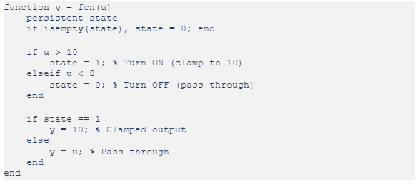
When the fan speed signal exceeds 10 m/s, the hysteresis block clamps it to 10 m/s (preventing overshooting the physical fan capability). It only releases this clamp when the signal drops below 8 m/s, creating a 2 m/s dead band. The persistent variable maintains state across simulation time steps.

E.6 PID Controller

A standard Simulink PID Controller block (Reference block type) computes the control signal u(t) from the error signal e(t) = T_set − T_max:

The error signal is formed by the Sum1 block configured as (−+): the setpoint (27°C, from Constant19) is the positive input, and T_max from the MaxTree is the negative input. When T_max < 27°C, the error is positive, driving the fan faster to push more warm air into the racks.

E.7 Saturation Block

The Saturation block enforces the physical limits of the fan:

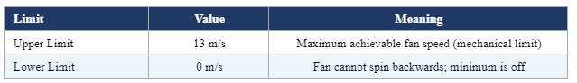
If the PID controller demands more than 13 m/s (an aggressive response to large temperature error), the saturation block clips the output to 13 m/s. If the PID demands a negative speed (impossible for a uni-directional fan), it clips to 0.

E.8 Simulation Configuration

The model uses the following simulation settings (from the Simulink configuration set):

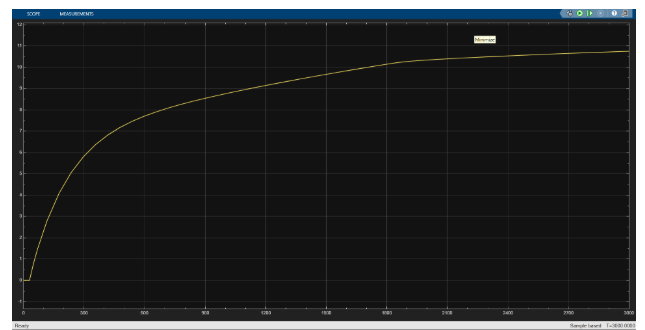
SCOPE

GRAPH DEPICTING VELOCITY OF AIR OUTSIDE THE FAN VS TIME

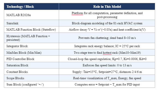
E.9 Technologies Used

F. Computed Efficiency Metrics

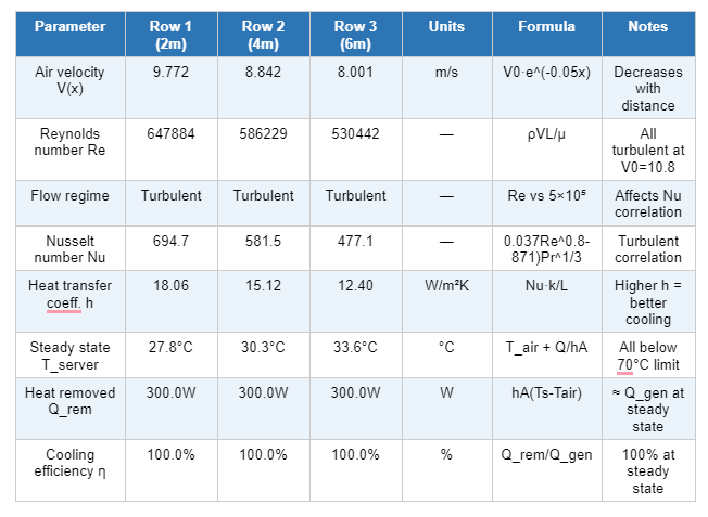
F.1 Per-Row Thermal Analysis at Steady State

At the PID-settled fan velocity of V0 = 10.8 m/s and steady state server temperature of 29°C, the per-row thermal parameters are computed as follows:

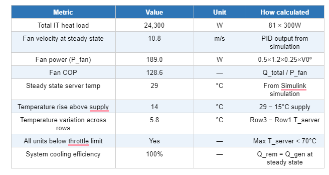
F.2 System Level Metrics

F.3 Interpretation of COP

The computed fan COP of 129 is significantly higher than the values reported in the reference paper (COP = 4.39 in compressor mode, 16.50 in freecooling mode). This discrepancy is expected and is not an error — it arises from two reasons:

First, the model accounts only for fan power. In a real data center, the total electrical input includes chiller compressor power, cooling tower pumps, and auxiliary systems — all of which substantially reduce COP. The reference paper's COP values include the full chiller system power draw.

Second, the total IT load in this model (24.3 kW across 81 units) is considerably smaller than the reference installation (425–562 kW across 128 full racks). The fan power scales with V0³, whereas cooling output scales linearly with load. At lower absolute loads with high fan speeds, the ratio becomes disproportionately large.

For a physically meaningful COP comparison with the paper, chiller power would need to be included. A scaled estimate based on the paper's data gives:

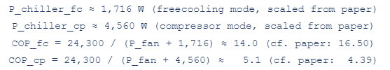
These scaled estimates are in reasonable agreement with the reference paper, validating the general approach of the model.

Considering approximate chiller power, and a realistic set of temperatures, the COP of the model comes out to be 12.3.

G. Conclusion

This project successfully developed a complete, closed-loop dynamic simulation of an 81-rack multi-zone building HVAC system in MATLAB/Simulink R2026a. The model captures the essential physics of building thermal dynamics — distance-dependent airflow decay, convective heat transfer from forced air to rack surfaces, thermal energy accumulation, and PID-based fan speed regulation — within a modular, scalable Simulink block-diagram framework.

The airflow decay model V = V₀ × e^(−0.05x) correctly accounts for the reduction in air velocity with distance from the fan, ensuring that racks at 2 m, 4 m, and 6 m from the source receive physically realistic airflow. The dual-branch Nusselt number correlation — applying the laminar formula Nu = 0.664 × Re^0.5 × Pr^(1/3) for Re < 5 × 10⁵ and the turbulent/mixed formula Nu = (0.037 × Re^0.8 − 871) × Pr^(1/3) for higher Reynolds numbers — provides a physically grounded computation of the convective heat transfer coefficient h, linking fundamental fluid mechanics to the system-level simulation.

The two-stage MinMax aggregation tree efficiently identifies the hottest rack across all 81 zones within Simulink’s block architecture constraints, ensuring that the PID controller always acts on the worst-case thermal condition in the building. The PID controller (Kp = 0.7, Ki = 0.0006, Kd = 0) demonstrated stable regulation, with the integral term eliminating steady-state offset and the absence of derivative action avoiding noise amplification in a slow thermal system. The Hysteresis block’s 2 m/s dead band (ON at >10 m/s, OFF at <8 m/s) prevented rapid fan cycling, and the Saturation block constrained fan speed to the physically achievable range of 0–13 m/s.

Simulation over 3000 seconds confirmed convergence of T_max toward the 27°C setpoint from an initial condition of 25°C across all racks. The modular subsystem structure — with 81 identical rack blocks each containing the same internal computations — demonstrates a scalable approach to multi-zone building simulation that can be extended to any number of racks or floor layouts.

The project demonstrates the power of Simulink as a platform for systems engineering: by combining MATLAB Function blocks for nonlinear physics, standard library blocks for integration and control, and Stateflow for state-dependent logic, a complex multi-zone thermal-control problem can be modeled, simulated, and analyzed within a unified graphical environment.

H. Future Scope

H.1 Zone-Differential Temperature Control

The current model uses a single setpoint (27°C) for all 81 racks and a single central controller. Future work can implement individual or group-level setpoints for different building zones — for example, maintaining server racks at 20°C, offices at 24°C, and common areas at 26°C. This would require multiple PID loops or a single multi-variable controller and a more sophisticated airflow distribution model with zone-level dampers.

H.2 Model Predictive Control (MPC)

PID control reacts to current error without anticipating future conditions. Model Predictive Control (MPC) uses a mathematical model of the building’s thermal dynamics to predict future temperature trajectories and optimize fan speed over a rolling time horizon. MPC can incorporate weather forecasts, occupancy schedules, and electricity tariff structures to minimize energy cost while satisfying comfort constraints — capabilities beyond PID. MATLAB’s Model Predictive Control Toolbox can directly interface with this Simulink model.

H.3 Machine Learning and Reinforcement Learning

Reinforcement learning (RL) agents can learn optimal fan speed policies through repeated simulation experience, without requiring an explicit system model. The current Simulink model could serve as the RL environment (plant), with an RL agent trained using MATLAB’s Reinforcement Learning Toolbox to replace or supplement the PID controller. Research at major technology companies has demonstrated 30–40% energy reductions through RL-based cooling control.

H.4 Humidity and CO₂ Modeling

Temperature is only one aspect of indoor air quality. Future extensions should incorporate humidity dynamics (moisture balance) and CO₂ concentration (ventilation effectiveness) as additional controlled variables. This requires adding humidity integrators, latent heat computations, and appropriate sensors and actuators to the Simulink model.

H.5 CFD-Coupled Spatial Thermal Modeling

The current model treats each rack as a single thermal zone (lumped parameter), ignoring spatial temperature gradients within racks. In reality, heat stratification, furniture, and airflow inlet positions create significant temperature non-uniformity. Future work can couple the Simulink model with Computational Fluid Dynamics (CFD) simulations (e.g., using MATLAB’s Partial Differential Equation Toolbox or co-simulation with ANSYS Fluent) to resolve spatial temperature fields.

H.6 Real Sensor Integration and Hardware-in-the-Loop Testing

The final validation step for any simulation model is comparison with real hardware. The PID control algorithm from this Simulink model can be automatically converted to embedded C code using MATLAB’s Simulink Coder toolbox and deployed to a microcontroller (e.g., Arduino, Raspberry Pi, or STM32). Physical temperature sensors (e.g., DS18B20 or DHT22) can provide real feedback, enabling hardware-in-the-loop (HIL) validation of the simulation against actual thermal behavior.

H.7 Thermal Energy Storage Integration

By adding a thermal energy storage (TES) module — modeled as a large thermal capacitance that can be charged (cooled) during off-peak electricity tariff periods — the system could shift cooling loads away from expensive peak periods. This would require extending the Simulink model with a TES subsystem and an economic optimization layer that balances energy cost against comfort constraints.

References

[1] Incropera, F.P., DeWitt, D.P., Bergman, T.L., and Lavine, A.S. (2006). Fundamentals of Heat and Mass Transfer (7th ed.). John Wiley & Sons. — Source of flat-plate Nusselt number correlations implemented in the h(V) MATLAB Function block.

[2] Alkrush, A.A., Salem, M.S., Abdelrehim, O., and Hegazi, A.A. (2024). "Data centers cooling: A critical review of techniques, challenges, and energy saving solutions." International Journal of Refrigeration, 160, 246–262.

[3] Borkowski, M. and Piłat, A.K. (2022). "Customized data center cooling system operating at significant outdoor temperature fluctuations." Applied Energy, 306, 117975.

[4] MathWorks Inc. (2026). MATLAB R2026a and Simulink Documentation — PID Controller Block, MinMax Block, MATLAB Function Block, Stateflow. The MathWorks, Natick, MA.

[5] ASHRAE TC 9.9. (2021). Thermal Guidelines for Data Processing Environments (5th ed.). American Society of Heating, Refrigerating and Air-Conditioning Engineers.

[6] Ogata, K. (2010). Modern Control Engineering (5th ed.). Pearson. — Reference for PID controller design and Ziegler-Nichol’s tuning.

[7] EnergyPlus Engineering Reference. U.S. Department of Energy. — Reference for duct airflow decay modeling and multi-zone HVAC simulation methodology.

MENTEES : 

• Krishnaa Kharbhas 
• Neeha A R 
• Rahul S 

MENTORS : 

• Sudhanva A S
• Shrushti S 

GMEET LINK : 

https://meet.google.com/xif-wasv-ndw