Aim:

Utilizing machine learning techniques to improve the performance and stability of Solid Oxide Fuel Cells (SOFCs)

Introduction:

A fuel cell is an electrochemical cell that converts the chemical energy of a fuel, typically hydrogen, directly into electrical energy using an electrochemical reaction with an oxidising agent, usually oxygen air.

SOFC is a fuel cell with a solid oxide as an electrolyte. At the cathode, the oxygen reduction reaction takes place. At the anode, the oxidation of oxygen from the electrolyte takes place. It runs at a temperature between 800-1000꠶C and can operate on hydrogen, hydrocarbons, natural gas and biofuels. SOFCs find their use in stationary power plants and auxiliary power supplies.

It has four types of cell designs: cathode-supported, electrolyte-supported, anode-supported and externally supported. The main factor in all these designs is the thickness of one of the components, specific to the cell design, be greater than the others.

The models created, analysed and studied in this project pertain to the anode-supported SOFC.

Experimental Procedure:

The project focuses on the impact of various parameters on the ohmic area-specific resistance (ASR) in the context of a solid oxide fuel cell (SOFC). In the experimental setup, each cell comprises five distinct layers: a porous Ni + YSZ anode support, a porous Ni + YSZ anode interlayer, a dense YSZ electrolyte, a porous LSM + YSZ cathode interlayer, and a porous LSM current collector. The ASR, denoted as Ri, is expressed as a function of the thicknesses of the electrolyte, electrodes, and potential interfacial resistances. When a single parameter, such as the thickness of a layer, is varied, the resistance dependence can be attributed solely to that layer's resistivity. For instance, varying the YSZ electrolyte thickness allows for the assessment of its influence on ASR. However, it's noted that observed variations may also result from unintended differences in other layers or contributions from sources other than the electrolyte. A linear relationship between ASR and electrolyte thickness is expected, with the slope representing the electrolyte ionic resistivity and the intercept indicating other sources of ohmic contribution. Experimental data confirm this trend, with measured ASR showing good agreement with reported values for YSZ electrolyte resistivity. Additionally, plots of ASR versus anode support thickness reveal the electronic resistivity of the anode support, providing further insights into SOFC performance. These findings underscore the complex interplay of different parameters and their effects on ASR, highlighting the importance of comprehensive analysis in optimizing SOFC design and performance.

Formulas and Models:

The effective anode support and anode interlayer diffusivities are respectively, Deff(1) H2−H2O and Deff(2) H2−H2O, wherein it is assumed that the effective diffusivities are proportional to the H2–H2O binary diffusivity (DH2−H2O), volume fraction porosity, and inversely proportional to tortuosity factor. Since other effects, such as Knudsen diffusion are likely present, and the exact nature of tortuosity is unclear, in the above description the tortuosity factor is a merely phenomenological fitting parameter. In steady state, under the assumptions made, the partial pressures of hydrogen and H2O at the anode interlayer/electrolyte interface as a function of current density are given respectively, by:

Effective Diffusivity of Hydrogen

Model:

Effective Diffusivity of Water

Model:

For an anode-supported cell with a small cathode thickness,we can estimate the oxygen partial pressure (pO2) at the interface between the cathode current collector and cathode interlayer in a solid oxide fuel cell (SOFC). It introduces a formula to calculate pO2 based on various parameters such as the oxygen partial pressure in the oxidant, current density, temperature, and cathode thickness. Additionally, it ensures that the oxygen flux through the current collector and cathode interlayer remains constant. Finally, it presents a method to determine the cathode limiting current density, which corresponds to the lowest possible oxygen partial pressure at the interface between the cathode interlayer and electrolyte, using certain constants derived from relevant parameters.

Effective Diffusivity of Oxygen

Model:

The maximum possible current density is that corresponding to the lowest possible oxygen partial pressure at the interface between the cathode interlayer and the electrolyte, which is zero (although p O2 of course can never be exactly zero). 

Governing Equation

Integrating ML models : 

After obtaining the voltage values from the Simulink models, we compile it into a dataset with all the features included at all the set parameter values the model is tested at. To integrate this data into a Machine learning model with the end goal of obtaining an accurate predictive model, we follow the sequence of preprocessing of data, importing the regression models from Python libraries and feeding the data into these models, training and testing these models with numerous algorithms to finally settle on one with low error.

Preprocessing of Data : 

The dataset obtained from the source model could contain certain outlier values that disrupt the models accuracy by considering these values while training the model, therefore it is important to standardize the dataset to obtain normally distributed data points with zero mean and unit variance. Methods like Standard Scaler from the Scikit learn library are used for this task.

Standardization : 

The dataset attributes are divided into two groups, X and Y, with X containing the input features like temperature, ASL thickness, ASL porosity, EL thickness, CFL thickness and Current Density and Y containing the Voltage values. The Standard scaler is then used to standardize the features and plotted onto a correlation map to identify the the correlation between the features and the voltage.

Data Distribution after Standardization of Features

Feature Decomposition : 

After the normal distribution of data is achieved we work towards minimizing the correlation between features by reducing the components of data. This is done through the use of Principal Component Analysis in the Scikit library, which is mainly used for dimension reduction purposes. PCA transforms the features into a new components with minimum correlation while also retaining the same information available in the original features and then the new components data distribution are mapped using matplotlib.

Data distribution of decomposed features after using PCA

The Covariance between the components is mapped using the Seaborn library with the aid of heatmaps.

The correlation is mapped between -1 to 1 with -1 and 1 indicating a linear relationship between the components and the target while 0 indicates a nonlinear relationship.

Splitting Data into train and test data : 

The data is split into training data for the model to be trained on and then into testing data for it to be evaluated. The train_test_split function from Scikit-learn is used for this process. It splits the data in and 4:1 ratio where 80% of the data is used for training and 20% is used for testing.

Training and Testing Different Models : 

Various models were trained and tested using their data and their learning and validation curves were plotted along with their prediction error curves and their evaluation and error scores were calculated and compiled into the table below.

As we observe from the table, the most suited models are MLP regressor, GP regressor, KNN regressor with all having R2 score above 0.99.

The models along with their Learning and Validation curves and Prediction Error plots are provided below. 

These models were used to predict the behavior of the fuel cell at different operating temperatures and their plots came out as such

MLP Regressor :

Learning and Validation Curves of MLP Regression

Prediction Error of MLP Regression

Effect of Operating Temperature on current-dependency

GP Regressor :

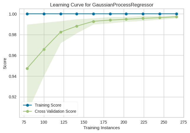
Learning and Validation Curves for GPR

Prediction Error of GPR

Effect of Operating Temperature on current-voltage dependency

KNN Regressor :

Learning and Validation Curves for KNN

Prediction Error of KNN

Effect of Operating Temperature on current-voltage dependency

Effect of CFL thickness on current-voltage dependency

Effect of Porosity on current-voltage dependency

Effect of anode support thickness on current-voltage dependency

Effect of electrolyte thickness on current-voltage dependency

Conclusion:

Machine Learning models have proven to be an excellent method of simulating and predicting the behaviour of fuel cells which are expensive to produce. We see that these models provide us with the best parameter values that can be used in our fuel cells without having to experiment with the proportions in the real world and with these 12 models tested to run predictions the K Nearest Neighbours model works best for our task with number of eighbours tested with set to 4.